|
Global curvature characterizes knot tightness. |
|
|
|
|
During a lunch-time discussion on the ideal shapes of knots and such, the concept of the "global curvature function" of a space curve was born. This function is related to, but distinct from, standard local curvature, and is connected to various physically appealing properties of a curve. Global curvature provides a concise characterization of curve thickness, and of certain ideal shapes of knots as have been investigated within the context of DNA. Moreover, global curvature is connected to the writhing number of a space curve and has applications in the study of self-contact and packing problems for rods. Some of the figures here are based on numerical data from
Katritch, V., Olson, W.K., Pieranski, P.,
Dubochet, J. & Stasiak, A.
(1997) Nature 388, 148-151.
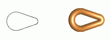
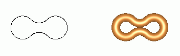
Any smooth, non-self-intersecting curve can be thickened into a smooth, non-self-intersecting tube of constant radius centered on the curve, as illustrated below.
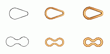
If the curve is a straight line there is no upper bound on the tube radius, but for non-straight curves there is a critical radius above which the tube either ceases to be smooth or exhibits self-contact. This critical radius is an intrinsic property of the curve called its thickness or normal injectivity radius. Of the two examples shown above, the first has a critical radius determined by smoothness
and the second has a critical radius determined by self-contact.
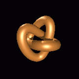
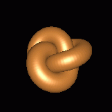
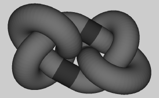
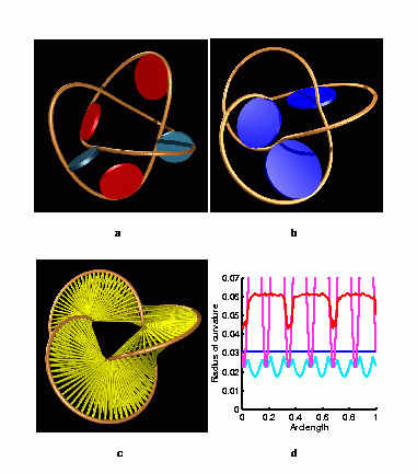
If one considers the class of smooth, non-self-intersecting closed curves of a prescribed knot type and unit length, one may ask which curve in this class is the thickest. The thickness of such a curve is an intrinsic property of the knot, and the curve itself provides a certain ideal shape or representation of the knot type. For example, the two curves shown below are of the same knot type (K31), but the second is substantially thicker than the first. In fact, the second is considered to be of maximum thickness for its knot type -- it is considered to be an ideal shape for the K31 knot.
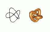
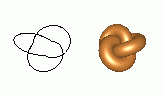
Approximations of ideal shapes in above sense have been found via a series of computer experiments by Katritch and coworkers. These shapes were seen to have intriguing physical features, and even a correspondence to time-averaged shapes of knotted DNA molecules in solution.
So how does one mathematically define curve thickness and the ideal shape of a knot? What are necessary and sufficient conditions for a knotted curve to be ideal? Answering these questions has led to a new geometrical quantity for space curves: the global radius of curvature function. This function provides a simple characterization of curve thickness, and provides an elementary necessary condition that any ideal shape of a knotted curve must satisfy. Moreover, global radius of curvature is connected to the writhing number of a space curve and has applications in the study of self-contact problems for rods.
Our definition of global radius of curvature is based on the elementary facts that any three non-collinear points x, y and z in three-dimensional space define a unique circle (the circumcircle), and the radius of this circle (the circumradius) can be written as
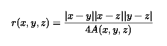
where A(x,y,z) is the area of the triangle with vertices x, y and z, |x-y| is the Euclidean distance between the points x and y, and so on. When the points x, y and z are distinct, but collinear, the circumcircle degenerates into a straight line and we assign a value of infinity to r(x,y,z).
When x, y and z are points on a simple, smooth curve C, the domain of the function r(x,y,z) can be extended by continuous limits to all points on C.
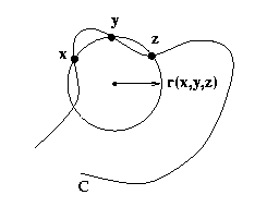
For example, the limit of r(x,y,z) as y,z approach x along C is just the standard local radius of curvature at x, and the limit circumcircle is just the osculating circle to C at x. If one holds x and y fixed, and takes the limit as z approaches y along C, then the limiting value of r(x,y,z) is the radius of that circle which passes through x and is tangent to C at y.
Given a simple, smooth curve C we define the global radius of curvature at each point x by
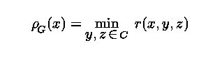
which can actually be shown to be a continuous function of x on C. Global radius of curvature can be interpreted as a generalization, indeed a globalization, of the standard local radius of curvature. In fact, since the points y=x and z=x are competitors in the minimization, global radius of curvature is bounded by local radius of curvature, that is,

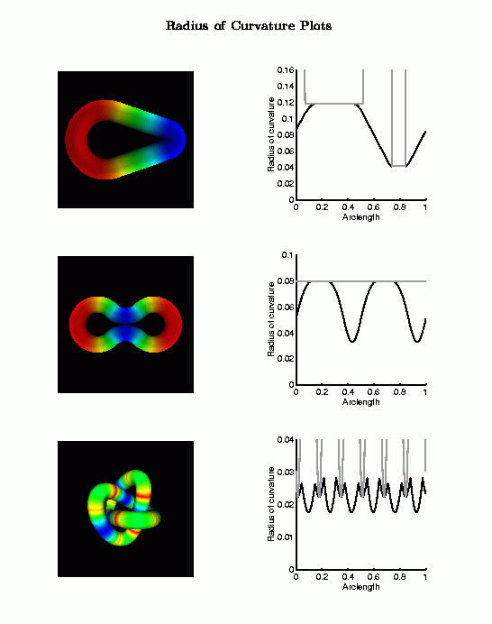
The figure below shows plots of global (black) and local (grey) radius of curvature versus arclength for some example space curves C. The space curves are represented by their critical tubes, which are colored by global radius of curvature. The blue regions are where global radius of curvature is minimal.

which is just the minimum value of the circumradius function r(x,y,z) over all triplets of points on C. This quantity has many physically appealing interpretations and applications:
We can now use rhoG(x) and Delta[C] to define and characterize ideal shapes of knots. Let K denote the set of smooth, non-self-intersecting closed curves of a prescribed knot type and length. Then a curve C* in K is ideal if and only if
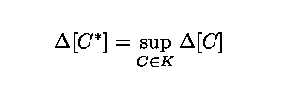
That is, among all curves in K, an ideal shape C* has maximal thickness. This definition corresponds precisely to the intuitive notion of the thickest tube of fixed length that can be tied into a given knot.
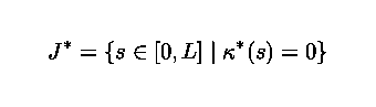
So what are the properties of curves C* that maximize Delta[C]? That is, what characterizes an ideal shape? Our study of this question led to the following theorem. Let C* be a curve in K with arclength parameter s in [0,L], and let J* be that subset of [0,L] for which the standard local curvature vanishes, that is
Then C* can be ideal only if there is a constant a>0 such that
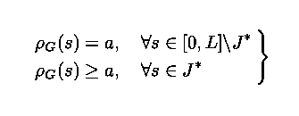
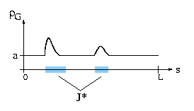
This constant a>0 is actually the thickness of the ideal shape -- it is the radius of the thickest tube of fixed length that can be tied into the given knot. While we have defined everything here for smooth curves, there is a straightforward extension to discrete (piecewise linear) curves.
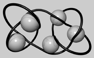
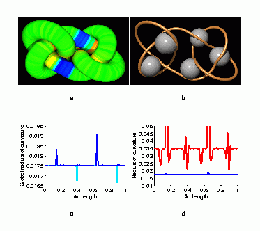
We tested our theorem on ideal shapes previously computed by A. Stasiak, V. Katritch and P. Pieranski. They had computed ideal shapes using hueristic, Monte Carlo type algorithms, and we had two main questions:
Results for non-ideal and ideal 3_1 knot
(new developments coming soon!)
(new developments coming soon!)