What is integration good for?

As we have seen, definite integrals can be used to compute area, just as derivatives can be used to compute slopes of tangent lines. But there is much more to derivatives than slopes of tangent lines, and there is much more to integrals than area. Integrals can be used to compute any bulk quantity.

Example: Distance

Suppose that we know a particle's velocity as a function of time. If the velocity is constant, then it's easy to find the distance traveled: $$ \hbox{Rate} \times \hbox{Time} = \hbox{Distance}.$$ If the velocity is almost constant, then we can get a good approximation by pretending that it is constant. If the velocity varies a lot, then we break our time interval into little sub-intervals on which the velocity doesn't change much, estimate each one, and add up the pieces. This is exactly the same strategy that we used for area under a curve.

Example 1: Find the distance traveled by a person walking at 2 MPH from 1:00 PM to 4:00 PM.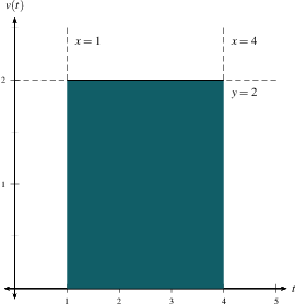 Solution: 3 hours at 2 MPH makes $3 \times 2 = 6$ miles.

Example 2: Find the approximate distance traveled by a person walking at velocity $v(t)=2 + 0.02 t$ MPH between $t=1$ (o'clock) and $t=4$ (o'clock). 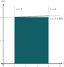Solution: The velocity doesn't change much between 1 and 4 PM, so we approximate our velocity as $v(1)=2.02$ and compute $(4-1)v(1) = 3(2.02)=6.06$ miles traveled.

The answer in Example 2 is a little bit too small, since the velocity goes up from $v=2.02$ at $t=1$ to $v=2.08$ at $t=4$. If we wanted an overestimate of the area, we would use the value of $v(t)$ at the right endpoint instead: $(4-1)v(4)=3(2.08)=6.24$. And if we wanted a more accurate guess, we might use the midpoint $f(2.5)=2.05$ and estimate the area as $(4-1)v(2.5)=3(2.05)=6.15$. But whether we use the left endpoint, the right endpoint, or the midpoint, we get roughly the same answer, since the velocity just isn't changing very much between $t=1$ and $t=4$.

By now you've probably noticed that this is exactly like finding the area under $y= 2 + 0.02x$ between $x=1$ and $x=4$. Only, in this case, the function is $v$ instead of $f$, and the variable $t$ instead of $x$, but it's the same calculation.

In general,